Performing adjoint optimization in Khepri. For starters, we are just optimizing a uniform slab.
Inverse design techniques are very popular now in electrodynamics. Inverse design aims to produce designs $\vec p$ that minimize some $f(\vec p)$, often called loss or figure of merit. I usually rely on heuristic methods which are, in a nutshell, smart ways to randomly sample the space containing $\vec x$, usually $\mathbb{R}^N$. Among inverse design methods we also find the adjoint optimization method. This method optimizes designs much like a neural network optimizes its parameters during training. Adjoint optimization is however extremely efficient as it doesn't rely on automatic differentiation. In brief, this method uses two simulations, one forward and an adjoint to compute the gradient of $f(\vec p)$ relative to the design parameters.
In this issue, we will consider that the figure of merit is the intensity of the electric field at some spot in the simulation $$ f(\vec p) = |E(\vec p)|^2=E\cdot (\delta \odot E)^\dagger $$ where $E$, without the vector notation is a supervector containing all field values. In practice, it is a table packing all field values $$ E = \left[E_x(\vec r_0), E_y(\vec r_0), E_z(\vec r_0), E_x(\vec r_1), \ldots\right], $$ where $\left\{\vec r_i, i=0, \ldots N\right\}$ are the sampling points of the fields. $\delta$ is a measurement mask that is zero everywhere except where we want to measure the fields so that they contribute to $f$. In our case, we consider that $\delta$ is only equal to one for $E_x$ and for a single point.
The first thing to do in order to perform gradient based optimization is to find an expression for the derivative of the figure of merit relative to the parameters vector $\vec p$
$$\frac{df}{d\vec p} = \frac{\partial f}{\partial E}\frac{dE}{d\vec p}+\frac{\partial f}{\partial E^\star}\frac{dE^\star}{d\vec p}=2\Re\left[\frac{\partial f}{\partial E}\frac{dE}{d\vec p}\right].\tag{1}$$
In this expression, $\frac{\partial f}{\partial E}$ is usually an analytical expression like the norm of the Poynting vector or like in our example, the intensity of the fields over any spatial extent. Therefore, the first factor $\frac{\partial f}{\partial E}$ can be computed analytically or through automatic differentiation. The second factor $\frac{dE}{d\vec p}$ however demands more attention and requires the two simulations.
It is now useful to express Maxwell equations in Fourier space $$ \left[\nabla\times\nabla\times - k_0^2\varepsilon_r(\vec r)\right] \vec E(\vec r) = -i\mu_0\omega \vec J(\vec r),\tag{2} $$ where $\vec J$ represents sources, $\omega$ the pulsation and $k_0$ the wavevector. This expression is expressible as a inhomogeneous supervector linear system of the form $$ \Omega E=\alpha J.\tag{3} $$ By taking the derivative of this equation with respect to the design parameters, we obtain $$ \frac{d\Omega}{d\vec p}E+\Omega\frac{dE}{d\vec p}=0, $$ as the source term is independent of the parameters. Rearranging the terms leads to an expression for the derivative of the fields we look for $$ \frac{dE}{d\vec p}=-\Omega^{-1}\frac{d\Omega}{d\vec p}E, $$ assuming that $\Omega$ can be inverted. By substitution in eq. (1), the full gradient equation becomes $$ \frac{df}{dp} = -2\Re\left[\frac{df}{dE}\Omega^{-1}\frac{d\Omega}{dp}E\right]. $$ The adjoint simulation can be identified in the above expression as $$ E_\text{ADJ}^T=-\frac{df}{dE}\Omega^{-1} $$ $$ \Omega E_\text{ADJ}=-\frac{df}{dE}^T. $$ This adjoint simulation uses the right hand side of the last equation as source, using the same geometry. By identifying this adjoint simulation, we have $$ \frac{df}{dp} = 2\Re\left[E_\text{ADJ}^T\cdot\frac{d\Omega}{dp}\odot E\right]. $$ $E$ and $E_\text{ADJ}$ can be obtained by engineering two simulations as we will see below. $\frac{d\Omega}{dp}$ however requires the derivative of the Maxwell operator. Luckily, one can prove that given eq. (2), the derivative only preserves the second term of the operator as $\varepsilon$ is dependent on the parameters $\vec p$: $$ \frac{d\Omega}{dp} = -k_0^2\frac{d\varepsilon_r(\vec r)}{dp} $$ We will again consider a simple case where $\vec p=\left[p_0\right]$ is just 1D and $\varepsilon_r=p_0 ~\forall~\vec r$ and the derivative of $\varepsilon$ is therefore 1. This leads to $$\frac{df}{dp} = -2k_0^2\Re\left[E_\text{ADJ}^T\cdot E\right].$$
The code used in this section is available on github.
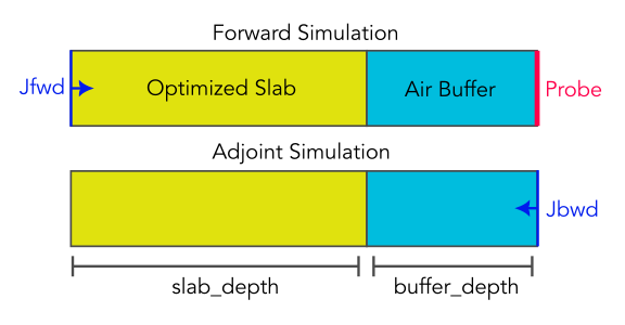
We will first tackle a simple problem: we are going to optimize the dielectric constant of a uniform slab ($\varepsilon_s$) to maximize its transmission ($S_{12}$). The incident beam has normal incidence and is polarized along x.
First, the forward simulation is set up for a reduced wavelength $\lambda=1.1$. Here, we only consider a uniform slab in the $X$ and $Y$ directions
from khepri import Crystal
import numpy as np

wavelength = 1.1
slab_depth = 0.7
buffer_depth = 0.5
def forward_cl(eps, wavelength, slab_depth):
    # Only (0,0) diffraction order is computed
    cl = Crystal((1,1))
    # The optimized slab
    cl.add_layer_uniform("U", eps, slab_depth)
    # We will need to compute fields too
    cl.set_device("U", fields_mask=True)
    cl.set_source(wavelength)
    cl.solve()
    return cl
There is not much to say about it, it is pretty standard, the only parameter being the $\varepsilon_s$ of the uniform slab. We also define a function for computing the adjoint crystal: it is reversed relative to the forward one:
def adjoint_cl(eps, wavelength, slab_depth, buffer_depth):
    cl = Crystal((1,1))
    cl.add_layer_uniform("U", eps, slab_depth) # Slab
    cl.add_layer_uniform("B", 1, buffer_depth) # Air buffer
    cl.set_device("BU", fields_mask=True)
    cl.set_source(wavelength) # We only set a wavelength
    cl.solve()
    return cl
The only original part is a $0.5a$ air buffer called B in front of the crystal. We will see why it exists in a few code blocks. The source is set without specifying a polarization as we will later use a specific value for the fields. Therefore, only $\lambda$ is set for now. The last function we need will compute the field $E_x$, where we need it. Notice how we override the incident wavevector of Crystal.set_source. This is because we need to use a specific value of the incident $E_x$ (source term $\alpha J$ in eq. (3)). To do so, we use the incident function to build a custom wavevector from a plane wave amplitude
Nslab = 64
from khepri.alternative import incident
def get_field(cl, zmin, zmax, source_x=1):
    x = y = np.array([0])
    x, y = np.meshgrid(x, y)
    z = np.linspace(zmin, zmax, Nslab)
    kz = 2 * np.pi / cl.source.wavelength
    efield = incident((1,1), source_x, 0,
    k_vector=(0, 0, kz), normalize=False)
    hfield = np.zeros_like(efield)
    # Call fields_volume with the override of incident fields.
    E, _ = cl.fields_volume(x, y, z,
    incident_fields=(efield, hfield)
    )
    # Only output Ex
    return E[:, 0, :, 0]
Finally, we can put everything together in the optimization loop:
from tqdm import trange
eps = 8
wavelength = 1.1
slab_depth = 0.7
buffer_depth = 0.5
arr0 = np.array([0])
k0 = 2 * np.pi / wavelength
lr = 0.9
profile, eps_vals = [], []
for i in trange(30):
    Efwd = get_field(clfwd := forward_cl(eps, wavelength, slab_depth), 0.01, slab_depth, 1)
    ex_probe = np.ravel(clfwd.fields_volume(arr0, arr0, [slab_depth+buffer_depth]))[0]
    Eadj = get_field(cladj := adjoint_cl(eps, wavelength, slab_depth, buffer_depth), buffer_depth, buffer_depth+slab_depth, np.conj(ex_probe))
    Eadj = np.flipud(Eadj)*1j
    dfdx = -2 * np.mean(np.real(Efwd*Eadj)) * k0**2
    eps_vals.append(eps)
    eps += lr**i * dfdx
    profile.append(np.abs(ex_probe)**2)
profile = np.array(profile)
From the above code, we see that we start with a value of $\varepsilon=8$, which is chosen because it is far from the optimum. The optimization is performed by gradient ascent, maximizing the value of the field at the probe point. Different archive arrays are used to track gradients, figure of merit and value of epsilon.
We can plot the different archives of performance using matplotlib.
import matplotlib.pyplot as plt
plt.style.use('seaborn-v0_8')
fig, ax1 = plt.subplots(1, 1, figsize=(4, 3), dpi=200)
ax1.plot(profile[:], label='Field probe / Fig. of Merit')
plt.legend()
ax1.set_ylabel("$|E_x|^2$")
ax1.set_xlabel("Iteration")
plt.legend(loc='best')
plt.tight_layout()
plt.savefig("adjoint_optimization.png")
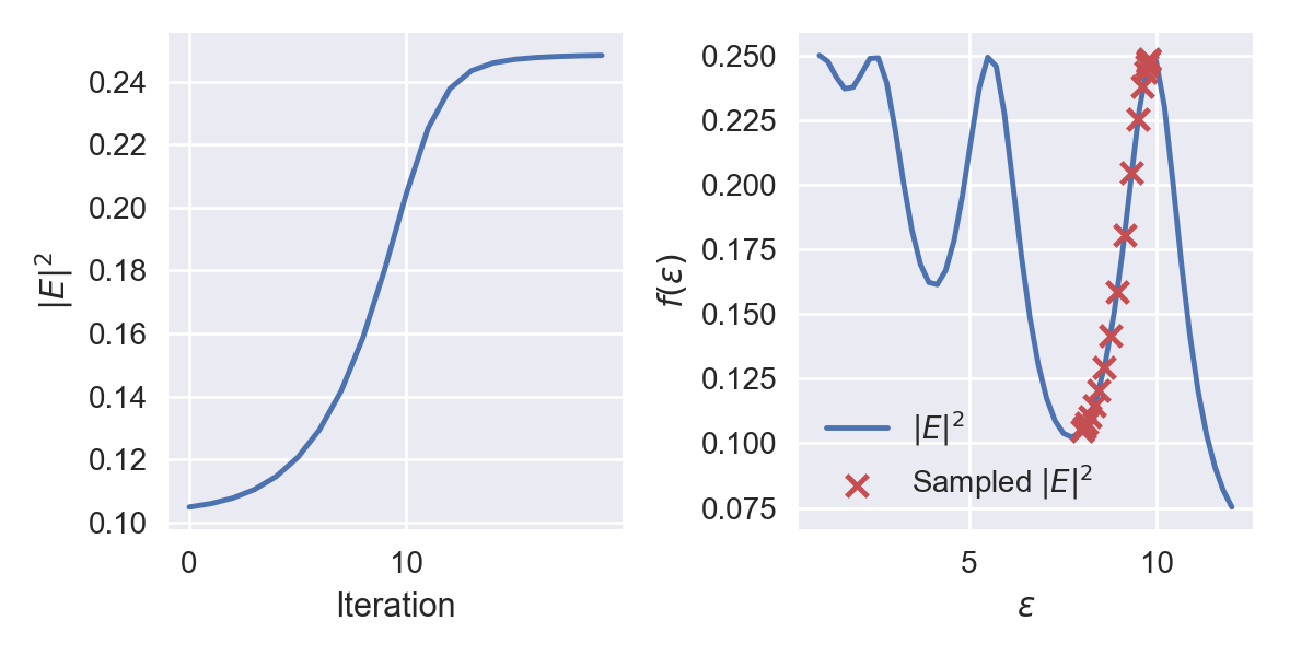
We obtain the following figures. In the left subplot, we show the figure of merit $|E|^2$ function of the optimizer iterations or epochs. As the optimizer iterates, we see this metric raising steadily to reach an optimum value of $0.25$ which corresponds to roughly $100\%$ transmission. On the right hand side, the figure of merit is charted for a wide range of $\varepsilon$. This figure therefore represents $f(p)$. We can do this as the problem has only one parameter and is extremely quick to evaluate. The red crosses represent the trajectory of the optimizer on this curve.
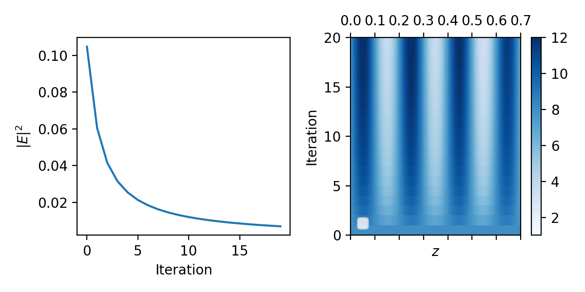
Now that we have a working implementation of the uniform slab, we can extend our implementation to $\varepsilon(z)$. Surprisingly, there is not much to do from our previous example.
The following figure shows on the left the figure of merit (minimizing field intensity) for 20 iterations. The map on the right shows the evolution of the z-varying dielectric profile from bottom (start) to top (finish). We start from an initial uniform slab and end up with a bragg mirror. Indeed, the resulting period is approximately $\Lambda\approx0.19$ in reduced units with a thinner high index region. The distributed Bragg mirror predicts a large photonic band gap $$ \frac{\Delta f_0}{f_0}=\frac{4}{\pi}\arcsin{\frac{n_2-n_1}{n_1+n_2}}\approx 1.28 $$ which is centered around, from eyeballing the figure,
$$ \frac{\lambda_\text{gap}}{4} = nd = n_1d_1+n_2d_2\approx0.05\times3.46+0.14\times1.0=0.313 $$ then $\lambda_\text{gap}\approx1.252$, which, given $\Delta f_0$ easily covers our wavelength $\lambda=1.1$.
We can observe the transmission spectra to convince ourselves.
Works, coming soon!
home