How to use my RCWA library to simulate displacement-sensitive photonic crystal slabs
All matters discussed in this tutorial post are extracted from this article written by Wonjoo Suh.
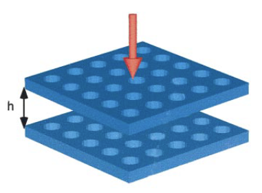
The structure consists in two stacked layers of dielectric constant \(\varepsilon=12\) separated by an air gap. The layers are \(0.55 a\) deep each and the air gap depth varies from \(0.55\) to \(1.35 a\) with \(a\) the lattice constant.
Our first objective is to reproduce Figure 2. We compute tranmission spectra for different interlayer depths.
We start by importing relevant modules and define the frequency range of interest:
from bast.alternative import scattering_layer, incident, Lattice
from bast.alternative import redheffer_product
import numpy as np
freqsn = np.linspace(0.49, 0.59, 100)
We define the parameters of the structures as described above
er  = 12
a   = 1          # We consider a case without dimensions
r   = 0.4        # Holes radius
d   = 0.55 * a   # Layer depth
his = [1.35,1.1,0.95,0.85,0.75,0.65,0.55]   # Interlayer depths
dis = [ hi * a for hi in his ]
We first draw our unit cell structure in a numpy array. The parameter N has no impact on the performance but it has to be high enough to get good fast fourier transform coefficients.
import numpy as np
N = 256
eps = np.ones((N, N))*er # Uniform dielectric
x = np.linspace(-0.5, 0.5, N)
y = np.linspace(-0.5, 0.5, N)
X, Y = np.meshgrid(x, y)
eps[np.sqrt(X**2+Y**2)< r] = 1.0 # Drilling the hole.
Now we devise a function to compute the scattering matrix of the system.
def get_smatrix(fn: float, di: float, pw=(9,9)):
    f = fn * c / a
    wavelength = c / f
    l = Lattice(pw, a, wavelength, kp=(0,0))
    # Our holey unit cell
    S = scattering_layer(l, eps, wavelength, a=a, depth=d)
    # A uniform air layer
    Si = scattering_layer(l, np.ones_like(eps), wavelength, a=a, depth=di)
    return redheffer_product(S, redheffer_product(Si, S))
Then we do a loop and compute all scattering matrice and their associeted transmissions.
kp = (0,0)
transmission_map = list()
for di in dis:
    for fn in tqdm(freqsn):
        S = get_smatrix(fn, di)
        f = fn * c / a
        wavelength = c / f
        k0 = 2 * pi / wavelength
        kzi = np.conj(csqrt(k0**2*epsi-kp[0]**2-kp[1]**2))
        T = compute_transmission(S, incident(pw, 1, 0, kp=(kp[0], kp[1], kzi)))
        transmission_map.append(T)

transmission_map = transmission_map.reshape(len(dis), len(freqsn))
Plotting this transmission_map gives the figure below.

home